SMPG Interface Overview

The SMPG tool consists of seven sections.

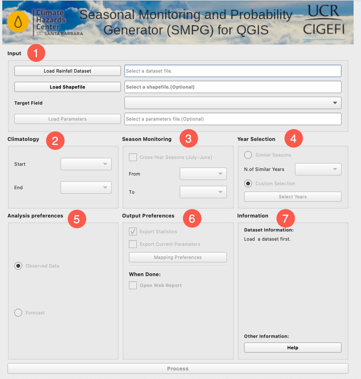
1. Input Section

The Input section is where users provide the primary datasets required for processing. This section includes the following fields:

• Time Series Table: The user must upload a table containing either the 5-day or 10-day total rainfall time series data for each polygon. This table should be generated as an output from GeoCLIM’s Extract Statistics function.

• Shapefile: The user must also upload the shapefile that was used to extract the rainfall data. This ensures the tool correctly maps the time series data to its corresponding polygons. If the user wishes to focus on a specific area within the larger region, a subregion of the original shapefile can also be used in combination with the same data table. This flexibility allows users to generate reports for targeted zones without needing to reprocess the entire dataset.

• Unique Identifier Field: Specify the field within the shapefile that uniquely identifies each polygon. This field ensures that the tool associates the correct time series data with each spatial unit.

• Reference Shapefile: Users may upload a reference shapefile that defines the full extent of the study region (for example, a nationwide shapefile). This file establishes the geographic framework within which the previously uploaded subregion shapefile can be aligned. By providing the complete-region shapefile, the tool can accurately position and interpret the subregion boundaries.

• Load parameters (.json): After completing all the required parameters for running the SMPG tool, users can save these settings for future use. This feature enables the tool to automatically load previously saved parameters, streamlining subsequent runs and ensuring consistency in the analysis. Users can revisit saved configurations to replicate workflows without manually re-entering inputs.

2. Climatology

In the Climatology section, users define the period that will be used to calculate the climatology or long-term mean (LTM), which serves as the baseline for identifying deviations from typical seasonal rainfall patterns. The selected period serves as the baseline for computing the following:

• Anomalies:
  Deviations from the long-term mean, indicating whether current rainfall amounts are above or below average.

• Percent Anomalies:
  The percentage difference between current rainfall and the climatological baseline.

3. Season Monitoring 

In the Season Monitoring section, users define the start and end of the rainy season to be monitored:

• Start of the Season (SOS):
  Specify the average start period for the season. It is recommended to include 2–3 periods prior to the expected SOS to allow the tool to identify early starts.

• End of the Season (EOS):
  Specify the expected end date for the season. This parameter enables the tool to make projections for the remainder of the season.

• Cross-Year Season (e.g., July–June):
  For seasons that span across two calendar years, users should select the Cross-Year Season option. When this box is checked, the tool reconfigures the period selection interface, allowing users to accurately define the start and end dates for cross-year seasons.

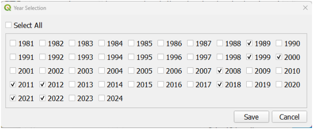
4. Year Selection

The Year Selection section allows the users to choose historical years to be used for completing the season from the current period to the End of Season (EOS). This process generates possible scenarios by combining the current season’s observed data (from the Start of Season, or SOS, to the current period) with historical data from each of the selected years. By using these historical patterns, the tool provides a range of potential outcomes for the remainder of the season, offering valuable insights for scenario planning and decision-making. The figure below shows a set of analog years selected. 

5. Analysis Preferences

In this section, users define the configuration of the analysis, determining whether it includes forecast data or relies solely on observed data:

• Forecast Inclusion:
  When selected, the SMPG identifies the last column of the table as the forecast. The tool incorporates this forecast data into the analysis to provide additional insights.

• Observed Data Only:
  When selected, the tool assumes that all the columns contain current data, no forecast. The analysis will be based solely on observed data up to the current period. 

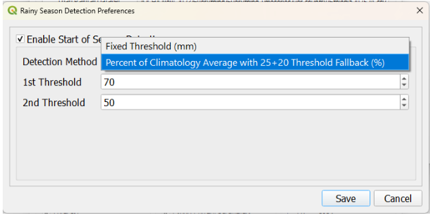
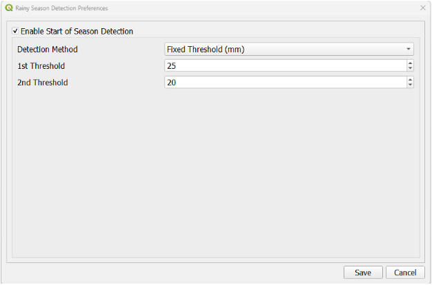
• Rainy Season Detection:

6. Output Preferences

In this section, users select the types of outputs generated by the tool. These options include the following:

• Export Statistics:
  Allows exporting the needed raw values of the computation. This is required to generate maps within QGIS (web report maps are not affected).

• Export Current Parameters:
  Users can save the parameters configured for the current analysis into a file. These saved parameters can be retrieved in Section 1 (Input) for consistent replication in future runs.

• Open Web Report:
  Allows to open the web report upon finishing the computation of the results.

• Mapping Preferences:
  By clicking the Mapping Preferences button, users can configure various map outputs, including:

  • C.Dk./LTA Pct.: Depicts the percent of the long-term average (LTA) for the accumulated precipitation from the Start of Season (SOS) up to the current period (current dekad: C.Dk.).

  • C.Dk. + Forecast/LTA Pct.: Depicts the percent of average for the accumulated precipitation from the Start of Season (SOS) up to the current period, including the forecast.

  • Current Season Pctl.: Shows the percentile rank of the accumulated precipitation from the SOS up to the current period, based on historical data.

  • Ensemble Med. Pctl.: Depicts the percentile rank of the median value of all possible outcomes at the End of Season (EOS). The ensemble is created using historical data from selected years (from Section 4) to simulate a range of potential outcomes.

  • Ensemble Med./LTA Pct.: Displays the percent of average for the EOS median value of all possible outcomes compared against the long-term average (LTA).

  • Tercile Probabilities: This map displays the probability of the season’s outcome falling into one of three categories:

    • Below Normal: Below the 33rd percentile of the historical distribution.

    • Normal: Between the 33rd and 67th percentiles.

    • Above Normal: Above the 67th percentile of the historical distribution.

    Each tercile category is displayed in a separate map, allowing users to view the probability associated with each possible seasonal outcome.

  • Start of Season (SOS): These maps show when the start of a rainy season has begun. The results of these maps depend on the selected method, and its parameters. These maps will be available only if Start of Season Detection is enabled.

    The maps produced for these data are the following:

    • Start of Season Class: This map shows when an SOS has been detected (for instance: Mar-1)

    • Start of Season Anomaly Class: This map shows how many periods the Start of season differs from the average (for instance: 2 Dekads Early).

7. Information

This section details key attributes of the input dataset, including the starting/ending years, the number of periods in the current year, and other relevant parameters.