Chapter 9: Background-Assisted Station Interpolation for Improved Climate Surfaces (BASIICS)

Summary

Satellite data provide useful information on climate variables (rainfall, temperature, and evapotranspiration) patterns. However, sometimes, satellite-estimated data contain biases and inaccuracies due to incorrect or limited ground data used during calibration. Some raster data also have a low spatial resolution, meaning the size of the pixel is too large for the area of interest. Such data could be improved by combining them with ground station information using the Background-Assisted Station Interpolation for Improved Climate Surfaces, (BASIICS) algorithm in GeoCLIM. See icon in red box in Figure 9‑1.

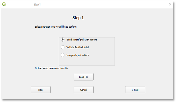
The BASIICS tool includes the following processes as shown in Figure 9‑2:

• Blend climate raster/grids with stations (BASIICS)

• Validate satellite data using ground station values

• Interpolate stations only

The following three-step process is recommended to produce improved gridded datasets:

1. Use the download function or import the raster datasets to be improved, see chapter 2.

2. Use the Validate Satellite Rainfall to determine if the satellite and station data are correlated.

3. If they are correlated, blend the two datasets to produce improved rainfall estimates. Save the settings to a file so you could use it later to update the improved rainfall times series.  

9.1. Validate satellite-based rainfall

The Validate Satellite Rainfall option allows you to evaluate grid/raster datasets (e.g., satellite-based rainfall estimates) using discrete points in space (e.g., rain gauges). The validation helps to determine if the two datasets are correlated to help in deciding if the blending option can be used with the two datasets to improve the raster using the point values by a blending process. The validation process first extracts values from a raster/grid at all locations where the point data have valid values (i.e., non-missing values. Missing values can be specified in the inputs). The results are: 1) A shapefile with the points that were included in the process. 2) A field of the interpolated values. 3) A .csv table that contains the station values, the corresponding grid value together with diagnostic information on the least-squares regression between the observed/in situ data value at the points being evaluated and the extracted grid values along with an R-squared output value. Once the correlation has been determined, then the raster and station data can be blended into an improved dataset.

To validate raster data, follow the three steps below:

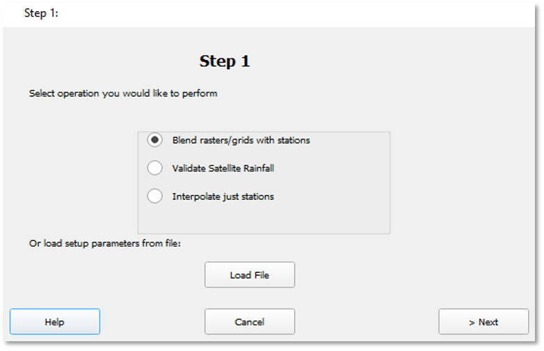
9.1.1. Step 1: Select the BASIICS option

1. Click on the BASIICS icon from the main toolbar to open the dialog box (Step 1) (Figure 9‑1).

2. Select the ■ Validate Satellite Rainfall option. See Figure 9‑2.

3. Click on the > Next button to proceed to Step 2.

9.1.2. Step 2: Dataset and station parameters

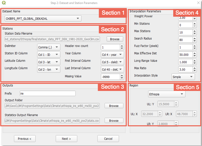
Complete the form with raster and station data information. This form is made of 3 sections, (Figure 9‑3).

9.1.2.1. Section 1: Grid Dataset Name

This section relates to the raster/grid input parameters. This process allows validation of climate datasets that have already been registered in GeoCLIM. To select the climate dataset to be validated, use the GeoCLIM dataset ˅ pulldown menu.

9.1.2.2. Section 2: Stations

This section relates to the station input parameters.

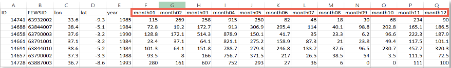
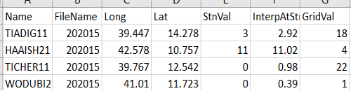
1. The tool assumes that all station data are in a single csv file. Browse to select the file that contains the station data. See an example in Figure 9‑4 of the file format. See the Data Management chapter for more information on the format of the table and other file types in GeoCLIM.

2. After selecting the station file, the tool identifies the header row and automatically completes the fields. Make any necessary changes to ensure that all field have the correct specification. When all the specifications are defined, move to section 3.

9.1.2.3. Section 3: Outputs

1. Specify the output prefix for all raster files created with the interpolation of the input stations.

2. Select the output folder.

3. Select the name for the statistics output file.

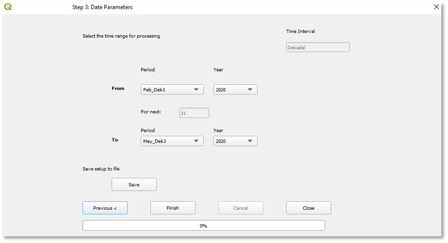
9.1.3. Step 3: Date parameters

Select the validation period as follows (see Figure 9‑5):

1. The time interval (e.g., month, dekad, or pentads) for the selected raster dataset is automatically displayed. Select the time range From and To of the raster data to validate. The time period and time interval are based on the selected climate dataset definition. In this example we are using dekads, see Figure 9‑5. And we are validating from (Feb dekad 01) to (May dekad 03), 2020.

2. Save the setup.  At this step, you can save the validation settings so you could open it from step 1, edit and reuse it.

3. Click on the Finish button to run the process.

Outputs: The validation process creates the following outputs:

1. A shapefile, for each period, containing all the stations that were used in the process.

2. An interpolated field, for each period, using the IDW process (see Figure 9‑6a).

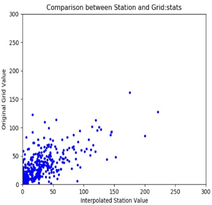
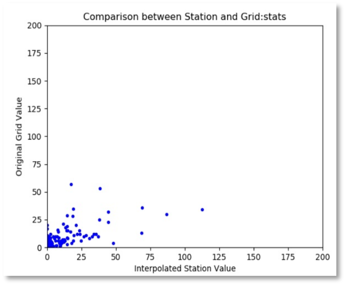
3. A scatterplot showing the satellite rainfall field values against the station values (Figure 96b).

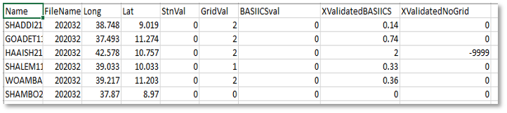
4. A CSV file with columns containing the metadata for each station together with the station value, the corresponding raster value, and the at-station interpolated value. These at-station interpolated values are produced to improve comparability between the gridded/raster data and the station data. The CSV file includes statistics showing the correlation of the rainfall field and station data (Figure 9-6c).

These outputs provide the basis to decide if it is appropriate to blend the stations and the raster datasets.

9.2. Creating Improved Rainfall Estimates (IRE) using BASIICS

Summary

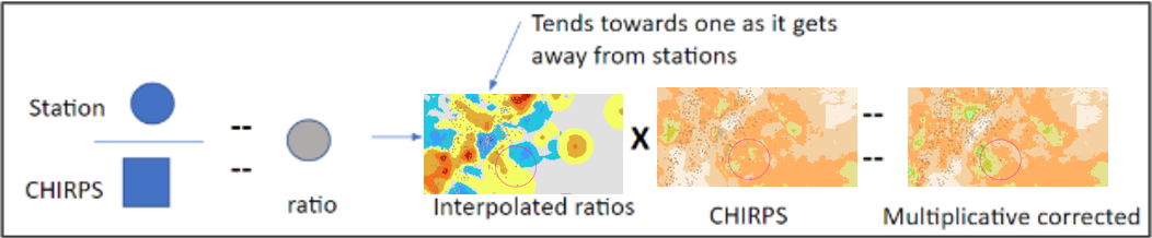
The Background-Assisted Station Interpolation for Improved Climate Surfaces (BASIICS) blending algorithm combines point rainfall observations (e.g., rain gauges) with a gridded background (e.g., satellite estimates such as CHIRPS) to produce an improved gridded rainfall field. 

At locations where stations overlap with the background grid, BASIICS extracts the pixel value corresponding to each station location. Two types of calculation are then made:

• Ratio = Station value ÷ Pixel value

• Anomaly = Station value − Pixel value

Both ratios and anomalies are spatially interpolated using a modified inverse-distance weighting (IDW) method that incorporates concepts from kriging. We will focus a big part of this chapter to understand the interpolation process. This produces two continuous fields: 

1. An interpolated ratio field 

2. An interpolated anomaly field

BASIICS then applies a two-step correction:

1. Multiplicative correction:
   Corrected = Interpolated Ratios × CHIRPS 

2. Additive correction:
   Final Estimate = Corrected + Interpolated Anomaly

The combination of these two corrections yields the final BASIICS rainfall estimate - also known as the Improved Rainfall Estimate (IRE) - which more closely reflects ground observations while retaining the spatial consistency of the background field.

9.2.1. Step 1: Select BASIICS option

1. Click on the BASIICS button from the GeoCLIM main toolbar.  See Figure 9-1.

2. Select the ■ Blend rasters/grids with stations option. At this point you can click on the Load File button to load previously saved settings or click on the > Next button to start a new blending process. See Figure 9-7.

9.2.2. Step 2: Dataset and interpolation parameters

The program expects two types of data as described below:

1. A point dataset with values at discrete locations in space (example: rain gauges) 

2. A grid dataset with values varying continuously over space (for example, a satellite-based rainfall estimate grid or a climatic average). For the algorithm to be used effectively, the two datasets need to be correlated. 

Complete the form with raster and station data information. This form is made of 5 sections, see (Figure 9-8). 

9.2.2.1. Section 1: Select the gridded climate dataset

This section relates to the raster/grid input parameters. This process allows the improvement of climate datasets that have already been registered in GeoCLIM. To select the climate dataset to be used in the blending process, use the Dataset Name ˅ pulldown menu.  In this example we are going to blend CHIRPS dekadal data with stations.

9.2.2.2. Section 2: Select station table

This section relates to the station input parameters.

The tool assumes that all station data are in a single csv file. Browse to select the file which contains the station data. See an example in Figure 9‑9 of the file format. The order of the columns is not important, but must include the following:

1. A unique station identifier ID, in a single column.

2. A column with longitude in decimal degrees.

3. A column with latitude in decimal degrees.

4. A column with year value (yyyy).

5. A series of consecutive columns for the number of periods (72 for pentads, 36 for dekads, or 12 for months). 

6. Any missing data should be completed with a single Missing Value, for example (-9999).

Once you select the station file, the tool identifies the header row and automatically completes most of the fields. Make any necessary changes to ensure that all fields have the correct specification. 

9.2.2.3. Section 3: Outputs

In the third section, you can specify the output directory where to save the blended products. At this point, you have two options: (1) create a new dataset or (2) update an existing dataset.

1. Create a new dataset: This first option allows you to create a new dataset in the correct format so it works with the GeoCLIM functions; for example, you are blending, for the first time, your stations with the historical data of CHIRPS or CHIRP and want to create a new dataset from the results. To do this:

   1. Provide a prefix for the output files.

   2. Browse to the GeoCLIM data repository. For example: X:~\fews_tools_WS\ProgramSettings\Data\Climate\new_dataset where X:~ is the path to your GeoCLIM workspace.

   3. The path on the Statistics Output Filename field changes automatically when you define the output directory.

   4. Make sure to complete the fields in sections 4 and 5 before continuing. (See sections 4 and 5 for complete explanation of the parameters).

   5. Click Next after completing all the fields.

   6. A dialog box appears asking Do you want to create a new dataset from outputs?

      1. Click on Yes.

      2. Enter a new name with no spaces.

      3. Select the data type.

      4. Select the extent of the data. If your region is outside of Africa or Central America, please select global.

      5. Click OK to move to Step 3.

2. Update an existing dataset: The second option is to add the latest record to an existing dataset. For example, you are blending the latest CHIRPS dekad with the stations and updating the time series you created previously.

   1. In the Output folder field, browse to the existing directory X:~\fews_tools_WS\ProgramSettings\Data\Climate\existing_dataset where X:~ is the folder containing the workspace.

   2. The path on the Statistics Output Filename field changes automatically when you specify the output directory.

   3. Make sure to complete the fields in sections 4 and 5 before continuing. (See sections 4 and 5 for complete explanation of the parameters).

   4. Click Next after completing all the fields.

   5. A dialog box appears asking Do you want to create a new dataset from outputs?

      1. Click on No to move to Step 3.

9.2.2.4. Section 4: The blending process - interpolation parameters

The program offers a set of options to adjust the parameters of the interpolation (Figure 9‑10).

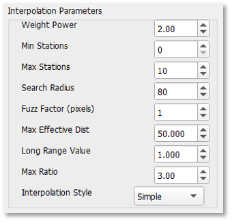
Make sure you fully understand these parameters before making any changes. Otherwise, it is recommended to leave the default values. A description of each parameter is provided below.

9.2.2.4.1. Weight Power (WEIGHTPOWER)

The weight power is the exponent applied to the inverse of the distance when calculating station weights, see Equation 9-1. It determines how quickly the influence of a station decreases with distance from the interpolation point, See Figure 9.11.

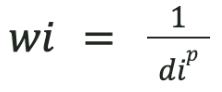
•  p = 0 → all stations have equal weight (no true interpolation).

• p = 1 → slow decay, distant stations still matter.

• p = 2 → faster decay, closer stations dominate.

• p ≥ 3 → very strong local influence, risk of bullseyes.

9.2.2.4.2. Search Radius, Min Stations, Max Stations

• SEARCHRADIUS: Maximum distance (in km) to search for stations around each pixel.

• MINSTNS: Minimum number of stations required for interpolation.

• MAXSTNS: Maximum number of stations allowed for interpolation.

At each pixel, the algorithm finds the nearest stations within the search radius. The number of stations used is limited between MINSTNS and MAXSTNS.

Example:
If SEARCHRADIUS = 200 km, MINSTNS = 2, and MAXSTNS = 10:

• If 7 stations are found within 200 km → all 7 are used.

• If fewer than 2 are found → the pixel will have a missing value.

To avoid missing values, it is recommended to set MINSTNS = 0, so that a value is always produced (with the background field filling gaps).

9.2.2.4.3. Fuzz Factor (FUZZFACTOR)

The fuzz factor generalizes the influence of stations to the pixel scale by introducing a small uncertainty in station locations.

• Distances are increased by (pixel size × fuzz factor).

• Prevents pixels containing a station from replicating the exact station value.

• Helps reduce the “bull’s eye” effect around stations.

FUZZFACTOR = 0→ pixels near a station are as close as possible to the station value.

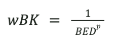
9.2.2.4.4. Background Equivalent Distance

The Background Equivalent Distance (BED) represents the assigned distance of the BK station that carries the value of the background raster (e.g., CHIRPS) at the pixel location.

• Smaller BED → stronger background influence (solution tends toward CHIRPS even near stations).

• Larger BED → weaker background influence (nearby stations dominate; background mainly anchors far from stations).

9.2.2.4.5. Long Range Value (LR_VALUE)

It is the value assigned to the BK station (the conceptual-station that represents the background field) which is placed at the BED distance from each pixel. The Simple interpolation starts by adding the BK station to the IDW process.

Where it applies

• Blending → Simple (idw_s): LR is the ratio value for the BK station.

• Interpolate Stations Only → Simple: LR is a constant baseline (there is no CHIRPS raster here); the BK station still uses LR at distance BED.

• Not used:Ordinary (idw_o) in either mode (no BED/LR term is added).

Units
None (ratio units). 

How it enters the interpolation (Simple style)
For a pixel x, a BK station with weight ​is added to the IDW process.

The value contributed by that station is:

• Ratio surface: value BK = LR

• Anomaly surface: value BK = 0 (baseline anomaly is zero)

After this seed term, nearby stations are added with their usual IDW weights.

Recommended settings (best practice)

• Ratio surface: LR = 1 (keeps background unbiased).

• Anomaly surface: LR = 0 (no additive bias).
  Changing LR away from these values overwrites the natural behavior:

• LR = 0 (ratio): suppresses the background (values collapse where no stations).

• LR > 1 (ratio): inflates remote areas toward LR (unphysical).

• LR < 1 (ratio): deflates remote areas.
  For these reasons, LR should normally remain at 1 (ratio) and 0 (anomaly).

9.2.2.4.6. Max Ratio (MAXRATIO)

The maximum ratio limits extreme values of the station/grid ratio used in the multiplicative correction.

• Ratio = Station value ÷ Grid value

• Large ratios can lead to exaggerated corrections when interpolated and applied to distant pixels.

Example:
Station value = 10 mm, grid pixel = 1 mm → ratio = 10.
If interpolated, this ratio could cause a nearby grid pixel of 30 mm to be scaled up toward 300 mm.

By default, MAXRATIO = 3, meaning any ratio > 3 is reset to 3. This prevents unrealistic “run-away” values. Users may adjust this threshold, but very high cut-offs are not recommended except for special cases.

9.2.2.4.7. Interpolation Style (INTERPOLATIONALGORITHM)

Two IDW algorithms are available:

• Simple (idw_s) → includes the background field (recommended/default).

  • BED is used.

  • The background pixel contributes as an additional weight.

  • Influence of the background increases as the distance to real stations increases.

• Ordinary (idw_o) → standard IDW.

  • Weights depend only on surrounding stations.

  • Background field does not contribute.

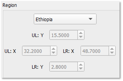
9.2.2.5. Section 5 Region - geographic location

Define Map Limits: Allows you to define the interpolation area (Figure 9-12).  Make sure that the area is smaller or equal to the gridded dataset. This area can be defined by using the extent of an existing GeoCLIM Region or other spatial data (raster or vector). This option helps to speed up the interpolation process.

To run the blending process, follow the steps below:

1. Choose the region from the list. 

2. Click on Next To move to step 3. 

9.2.2.6. Example: Estimating rainfall value at Location x

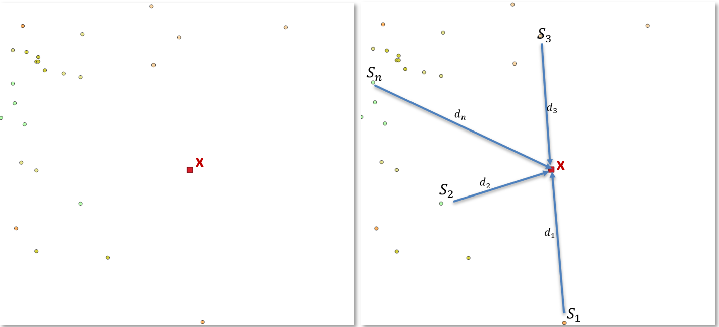
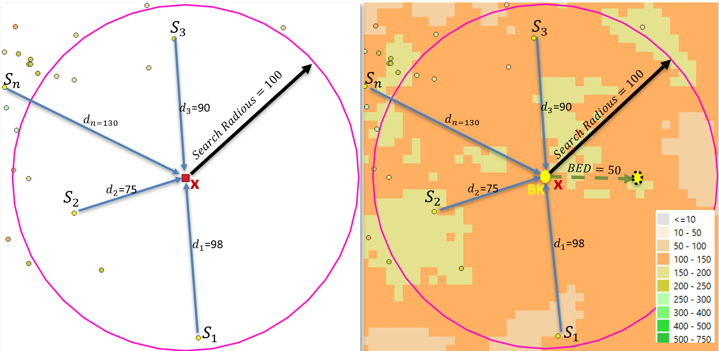
To illustrate how BASIICS works, we build an example step by step. We aim to estimate the rainfall at the target pixel x—shown in red in Figure 9-13 (left)—using the surrounding gauge stations. Each nearby station contributes its observed value Si​ and its distance to pixel x, di​, as depicted in Figure 9-13 (right). These distances are then used to compute station weights in the basic IDW interpolation; we examine this process in more detail in the next section.

What makes BASIICS different, however, is the inclusion of a background field, in this case CHIRPS. This background field is introduced through an imaginary background station (BK) placed at pixel x. This station is assigned a weight in the IDW process as if it were located at a fixed distance - the Background Equivalent Distance (BED) -. By doing so, BASIICS combines the influence of ground stations with the CHIRPS background field in a consistent interpolation framework.

9.2.2.6.1. Inverse Distance Weighting (IDW) and BASIICS Parameters

Let’s first see how regular IDW would deal with this example.

IDW interpolation estimates the value at an unknown point as a weighted average of nearby station values. The influence of each station decreases with distance: closer stations exert more weight, while distant stations contribute less. A maximum distance, or Search Radius, is typically specified to ensure that only stations within a practical range affect the interpolation.

See more about IDW here https://pro.arcgis.com/en/pro-app/latest/tool-reference/3d-analyst/how-idw-works.htm  

Formally:

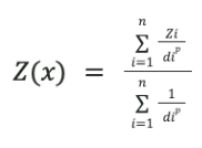
where:

• Z(x) = interpolated value at location x

• Zi​ = value at station i

• di = distance between location x to be estimated and station i

• p = weighting power (controls how quickly influence decreases with distance), see figure 9.11

The distance from each station to the location x, combined with the power P, is used to estimate the weight or in other words the influence each station will have in estimating x. Figure 9-11  shows the effect of the different P values in how fast the weight of the station value decreases with distance.

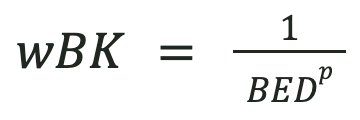
9.2.2.6.2. Incorporating the Background Field

Up to this point, we have illustrated a standard IDW interpolation, where the estimate at location x depends only on the surrounding stations, see Figure 9-14 left. In our case, however, there is an important difference:  We also have a background field — in this case, CHIRPS — which provides spatially continuous rainfall estimates, even in areas where no stations are available, see panel on the right on Figure 9-14. In this section we introduce two new concepts. The background (BK) station shown in yellow, and the Background Equivalent Distance (BED), see panel on the right on Figure-14. The main purpose of the BK station is to allow the background field to influence the interpolation process at each pixel, having a relatively stronger influence as surrounding stations become further than BED away from the pixel being interpolated to.

BASIICS is a modified IDW process that incorporates a background field by adding a conceptual (imaginary) station at every pixel x being estimated. We will refer to this conceptual station as BK (for BacKground). There is a BK station at every pixel x that we are estimating. Since all the stations in the process are assigned a weight based on their distance to the pixel x, the station BK also is assigned a weight as if it were at a distance BED. See right panel on Figure 9-14.  

9.2.2.6.3. Let’s summarize the BK station (Simple style)

• Location: BK is placed at the pixel x being estimated.

Weight: BK is given the IDW weight of a station located at the Background Equivalent Distance (BED):

• Value: BK represents the background field (e.g., CHIRPS).

  • In the ratio surface, BK’s value is the Long Range (LR) baseline, typically 1, which corresponds to CHIRPS/CHIRPS=1.

• In the anomaly surface, BK’s value is 0, which corresponds to CHIRPS−CHIRPS=0.

Role: BK anchors the interpolation so that, far from stations, ratios relax toward LR (=1) and anomalies toward 0, causing the final estimate to revert smoothly to the background.

9.2.2.6.4. Creating the Improve Rainfall Estimate (IRE)

As mentioned in the introduction to the BASIICS process, the Improved Rainfall Estimate (IRE) is produced through two main correction steps: multiplicative and additive. In this section, we focus on completing both steps by applying the framework and parameters discussed earlier—such as Search Radius, Minimum/Maximum Stations, Weight Power, BED, Long Range and background station, Max Ratio, and Fuzz Factor.

To begin, we perform the multiplicative correction by interpolating the required ratios across the spatial domain. These interpolated ratios are then used as input for the additive correction step, ensuring that both spatial and observational adjustments are applied effectively.

9.2.2.6.5. Multiplicative correction

This is the first step in adjusting satellite-based rainfall estimates, in our case CHIRPS, using gauge observations, see Figure 9-15. This step works by calculating the ratio between observed rainfall at stations and the corresponding CHIRPS pixel value, then interpolating these ratios across space to generate a correction surface. This surface is applied multiplicatively to the satellite data, effectively scaling the CHIRPS values to better match ground observations. The goal is to correct for systematic biases in satellite data before applying further local adjustments through the additive correction.

Let’s look at the Interpolating ratios process:

Definitions:

• R^(x) = interpolated ratio value at pixel x

• r_i= ratio at station i (station ÷ CHIRPS)

• w_i(x)=1 / d(p/i), IDW weight of station i at pixel x

• d_i = distance from pixel x to station i

• p = IDW power parameter

• w_BK​ = IDW weight of the background station (BK), always included

• LR = long-range ratio value assigned to BK (commonly set to 1)

An epsilon (ϵ) is used internally to avoid divide-by-zero.

BASIICS generates a continuous ratio surface across the domain. This surface is produced with a modified IDW scheme that respects the search radius and station-count constraints, caps extreme values using the Max Ratio setting, and includes the background pixel as a conceptual station (BK) in Simple mode. Far from gauges, ratios relax toward the Long-Range value (LR = 1), ensuring that the multiplicative correction remains unbiased where station influence is weak. Figure 9-16 below displays a typical interpolated ratio field. 

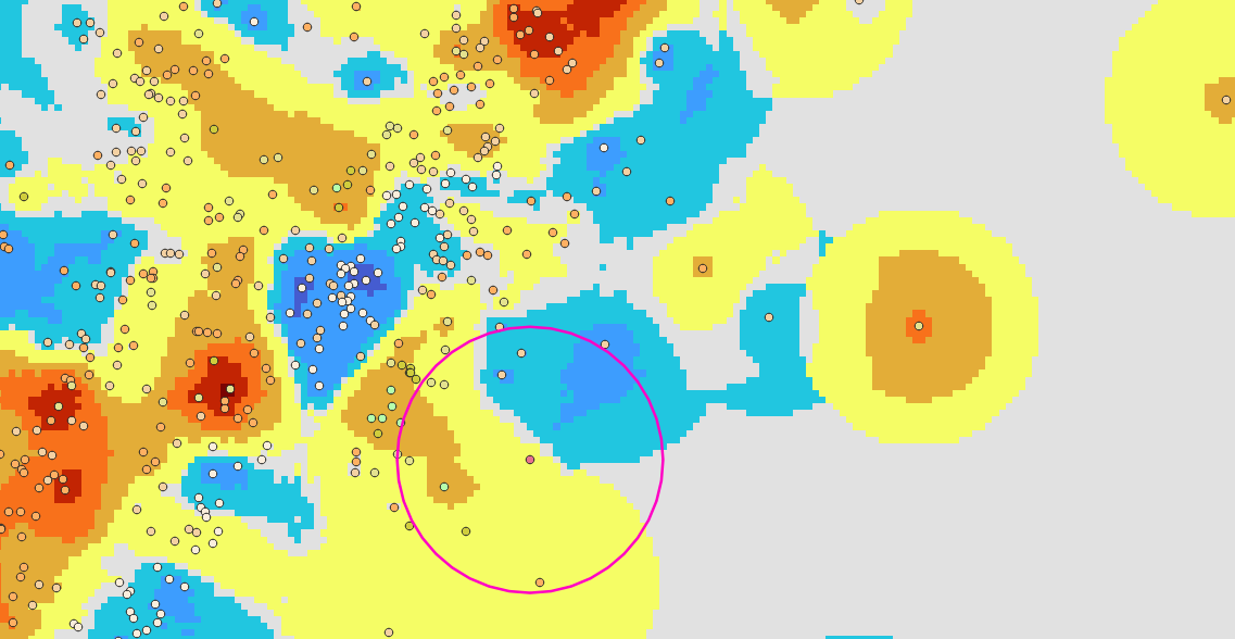
With the multiplicative correction applied, the large-scale bias between CHIRPS and station observations has been adjusted, producing a corrected rainfall field. However, local differences may still remain, as station observations can capture finer-scale variability that CHIRPS does not fully represent. To address this, we apply the additive correction, which incorporates station anomalies into the estimate.

9.2.2.6.6. Additive correction

This is the second step in the BASIICS process and is applied after the multiplicative adjustment. While the multiplicative correction removes large-scale biases between CHIRPS and station data, the additive correction focuses on reducing local differences. It does this by calculating anomalies (station − CHIRPS) at gauge locations, interpolating these anomalies across space, and then adding the interpolated anomaly field to the multiplicatively corrected rainfall. This step ensures that localized deviations captured by the stations are incorporated into the final estimate, improving spatial detail and accuracy in the Improved Rainfall Estimate (IRE). The workflow for this step, and its role in generating the final Improved Rainfall Estimate (IRE), is illustrated in Figure 9-17. 

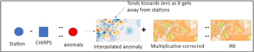
Interpolating anomalies

Definitions:

• Â(x) = interpolated anomaly value at pixel x

• a_i = anomaly at station i (station - CHIRPS)

• w_i(x) = 1 / d(p/i), IDW weight of station i at pixel x

• d_i = distance from pixel x to station i

• p = IDW power parameter

• w_BK = IDW weight of the background station (BK), always included

• 0⋅w_BK = background station anomaly contribution, which is always zero

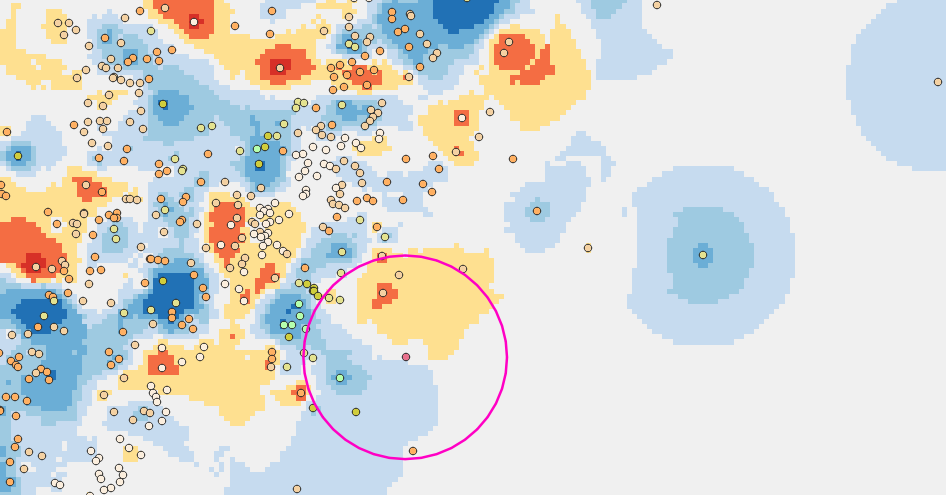
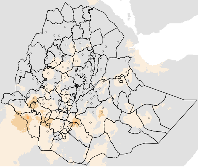
Once (station − CHIRPS) anomalies are computed, the same interpolation framework is applied to create a continuous anomaly surface. Close to gauges, the field reflects observed local departures; away from gauges, the field trends to zero, preventing artificial additive bias. This anomaly surface is then added to the multiplicatively corrected CHIRPS field to yield the final Improved Rainfall Estimate (IRE). The map on Figure 9-18 illustrates a typical interpolated anomaly field and the station distribution used in that period.

9.3. Step 3: Date Parameters and saving settings

To save the date parameters and settings follow the steps below (Figure 9-19):

1. The time interval (e.g., month, dekad, or pentads) for the selected raster dataset is automatically displayed. 

2. Select the time range From and To of the data to blend. The time period and time interval are based on the selected climate dataset definition. In this example we are using dekads, see figure 9-19. And we are blending from Feb (dekad 01) to May (dekad 03) 2020.

3. Save the setup.  At this step, you can save the blending settings so you could open it from step 1, edit and reuse it. 

4. Click on the Finish button to run the process.

9.4. Outputs

The blending process creates the following outputs:

1. A shapefile, for each period, containing all the stations that were used in the process.

2. The blended field, for each period. See Figure 9-16a.

3. The interpolated ratios and interpolated anomalies fields, for each period.

4. Three scatterplots showing the relationship of the original grid and the station values (Figure 9-16b) for example. 

5. A CSV file, (Figure 9-16c) containing the metadata for each station together with the following columns:

   1. Station value

   2. Corresponding raster value

   3. The BASIICS value at station location

   4. Cross-validated BASIICS value. Indicates the BASIICS value at the station location without including that specific station in the process. This value responses to the question, what would be the value at this pixel if the station were not there. 

   5. Cross validated interpolation only. Pixel value of interpolation of stations only, without including the corresponding station.

9.5 BASIICS Workflow 

This section describes the workflow outline based on documentation provided by the programming team. 

1. Read station file

   • Reads in the selected station file's data and splits it into two separate temporary CSV files:

     • "Region Stns" CSV: station ID, latitude, and longitude within the region’s extents.

     • "Region Data" CSV: data for each station within the region’s extents.

2. Generate station-to-station list

   • From the "Region Stns" CSV, generate stn_2_stn_list, where each index contains:
     [station, [ordered list (closest to furthest) of stations within search radius]]

3. Generate station-to-pixel list

   • From the "Region Data" CSV, generate stn_2_pixel_list, where each index contains:
     [[row of pixel, col of pixel], [ordered list (closest to furthest) of stations within search radius]]

4. Split data by period

   • From the "Region Data" CSV, split into separate CSV files for each period.

   • Store paths in split_csv_file_list.

5. Calculate Fuzzy Distance

   • Calculate and set the "Fuzzy Distance" from the "Fuzz Factor" for later IDW calculations.

6. Initialize stats file

   • Create stats.csv with header row.

7. Loop through each period

   1. Set base name for outputs (e.g., 2017.03.1 for 2017, March, dekad 1) (column B).

   2. Verify/get matching CSV for period from split_csv_file_list.

   3. Verify CHIRPS input grid file exists and return filename.

   4. Build station dictionary stn_dic from using outputs from steps b and c above:

      1. Keys = station ID (column A). Values = Longitude (C), Latitude (D), Stn_val (E).

      2. Set Grid_val (F) by reading in the CHIRPS file from step c and getting the value at station location.

   5. Interpolate station values using 'ordinary' type via cointerpolate_stations_idw, setting:

      1. Xvalidated_stn_val (I)

   6. Remove entries with missing data.

   7. Create station shapefile from stn_dic. From steps d,e,and f.

   8. Output initial stats to basiics_v2p0chirps<base_name>.stat.txt (first section: least squares stats comparing station values X and grid values Y).

   9. Calculate station ratios and add to stn_dic:

      1. Formula: (Interpltd_stn_val+ϵ)/(Grid_val+ϵ)(Interpltd\_stn\_val + \epsilon) / (Grid\_val + \epsilon)(Interpltd_stn_val+ϵ)/(Grid_val+ϵ) or Max Ratio if larger.

      2. ε = 10.0.

   10. Interpolate station ratios via cointerpolate_stations_idw, setting:

       1. Intrpltd_ratio_val

       2. Xvalidated_ratio_val

   11. Calculate Calculate the interpltd ratio and anom vals, this will set the "Int_ratio_x_grid_val", "Xval_ratio_x_grid_val", and "Anomaly_val"

       1. Int_ratio_x_grid_val = Intrpltd_ratio_val × Grid_val

       2. Xval_ratio_x_grid_val = Xvalidated_ratio_val × Grid_val

       3. Anomaly_val = Interpltd_stn_val − Int_ratio_x_grid_val

   12. Interpolate anomaly values via cointerpolate_stations_idw, setting:

       1. Interpltd_anomaly

       2. Xvalidated_anomaly

   13. Calculate Ratio + Anomaly, setting:

       1. Intrpltd_ratio_plus_anom = Int_ratio_x_grid_val + Xvalidated_anomaly

       2. Xvalidated_ratio_plus_anom_val = Xval_ratio_x_grid_val + Xvalidated_anomaly

   14. Start Blending steps:

       1. Interpolate station ratios to the pixel array → Interpolated Ratios Array → save as <base_name>_ratio.tif

       2. Multiply Interpolated Ratios Array × CHIRPS grid → Interpolated Ratios X Grid Array

       3. Extract values from Interpolated Ratios X Grid Array at stations → Interp_array_val

       4. Calculate anomalies: Interpltd_stn_val − Interp_array_val → Intrpltd_stn_minus_intrpltd_grid

       5. Interpolate Intrpltd_stn_minus_intrpltd_grid with simple IDW, relaxing anomalies to 0 farther from stations → anomaly array → save as <base_name>_anom.tif

       6. Final blended array = Interpolated Ratios X Grid Array + anomaly array → save as <base_name>.tif

   15. Extract values from final blended array at stations → final_basiics_val (G).

   16. Create <base_name>.crossval_graph.jpg:

       1. X: final_basiics_val (label: "BASIICS Pixel Value")

       2. Y: Xvalidated_ratio_plus_anom_val (label: "Cross-validated BASIICS Value")

   17. Create <base_name>.stngrid_graph.jpg:

       1. X: Intrpltd_ratio_plus_anom & final_basiics_val (label: "BASIICS Pixel Value")

       2. Y: Grid_val (label: "Original Grid Value")

   18. Output least squares stats (sections 2, 3, 4) with cross-validated stats to "base_name".stat.txt from step h

   19. PRINT OUT stats.csv here for all the station data columns above.

8. After loop completes

   1. Read back in stats.csv for all periods.

9. Create cumulative stats.crossval_graph.jpg

   1. X: column G (BASIICS Pixel Value)

   2. Y: column H (Cross-validated BASIICS Value)

10. Create cumulative stats.stngrid_graph.jpg

    1. X: column G (BASIICS Pixel Value)

    2. Y: column F (Original Grid Value)

11. Generate comparison statistics in stats.csv:

    • G vs F

    • G vs H

    • G vs I